6 Matrices
Operations
Matrices allow us to perform mathematical operations on many sets of numbers all at once. Because statistical analysis requires repeated calculations on rows and columns of data, matrix algebra has become the engine that underlies most statistical analyses.
6.1 Adding Matrices
In order to add or subtract matrices, they must be compatible, meaning that they must have same number of rows and columns.
To add compatible matrices, simply add elements in the same position.
\begin{aligned}\mathbf{A}+\mathbf{B}&= \begin{bmatrix} a_{11} & a_{12}\\ a_{21} & a_{22}\\ a_{31} & a_{32} \end{bmatrix}+ \begin{bmatrix} b_{11} & b_{12}\\ b_{21} & b_{22}\\ b_{31} & b_{32} \end{bmatrix}\\[2ex] &= \begin{bmatrix} a_{11}+b_{11} & a_{12}+b_{12}\\ a_{21}+b_{21} & a_{22}+b_{22}\\ a_{31}+b_{31} & a_{32}+b_{32} \end{bmatrix} \end{aligned}
If matrices are not compatible, there is no defined way to add them.
6.2 Subtracting Matrices
Subtraction with compatible matrices works the same way as addition—each corresponding element is subtracted.
\begin{aligned}\mathbf{A}-\mathbf{B}&= \begin{bmatrix} a_{11} & a_{12}\\ a_{21} & a_{22}\\ a_{31} & a_{32} \end{bmatrix}- \begin{bmatrix} b_{11} & b_{12}\\ b_{21} & b_{22}\\ b_{31} & b_{32} \end{bmatrix}\\[2ex] &= \begin{bmatrix} a_{11}-b_{11} & a_{12}-b_{12}\\ a_{21}-b_{21} & a_{22}-b_{22}\\ a_{31}-b_{31} & a_{32}-b_{32} \end{bmatrix} \end{aligned}
6.2.1 Adding and Subtracting Matrices in R
The R code for matrix addition and subtraction works exactly like scalar addition and subtraction.
6.3 Scalar-Matrix Multiplication
To multiply a scalar by a matrix, multiply the scalar by every element in the matrix:
\begin{aligned} k\mathbf{A}&= k\begin{bmatrix} a_{11} & a_{12} & a_{13}\\ a_{21} & a_{22} & a_{23} \end{bmatrix}\\[2ex] &= \begin{bmatrix} ka_{11} & ka_{12} & ka_{13}\\ ka_{21} & ka_{22} & ka_{23} \end{bmatrix} \end{aligned}
6.3.1 Scalar-Matrix Multiplication in R
To perform scalar-matrix multiplication in R, define a scalar, create a matrix, and then multiply them with the * operator.
k <- 10
A <- matrix(1:6,nrow = 2)
A
[,1] [,2] [,3]
[1,] 1 3 5
[2,] 2 4 6k * A [,1] [,2] [,3]
[1,] 10 30 50
[2,] 20 40 606.4 Matrix Multiplication
Matrix multiplication is considerably more complex than matrix addition and subtraction. It took me an embarrassingly long time for me to wrap my head around it. I will state things in the abstract first, but it is hard to see what is going on until you see a concrete example.
In order for matrices to be compatible for multiplication, the number of columns of the left matrix must be the same as the number of rows of the right matrix. The product of A and B will have the the same number of rows as A and the same number of columns as B.
Imagine that matrix A has n rows and m columns. Matrix B has m rows and p columns. When A and B are multiplied, the resulting product is matrix C with n rows and p columns.
\mathbf{A}_{n\times m} \mathbf{B}_{m\times p} = \mathbf{C}_{n\times p}
Element c_{ij} of \mathbf{C} is the dot-product of row i of \mathbf{A} and column j of \mathbf{B}. That is,
c_{ij}=\vec{a}_{i\bullet}\cdot\vec{b}_{\bullet j}
Figure 6.1 gives a visual example of matrix multiplication. Every row vector of A is multiplied by every column vector of B.
6.4.1 Matrix Multiplication Example
\mathbf{A}=\begin{bmatrix} \color{FireBrick}a&\color{FireBrick}b&\color{FireBrick}c\\ \color{RoyalBlue}e&\color{RoyalBlue}d&\color{RoyalBlue}f \end{bmatrix}
\mathbf{B}=\begin{bmatrix} \color{green}g&\color{DarkOrchid}h\\ \color{green}i&\color{DarkOrchid}j\\ \color{green}k&\color{DarkOrchid}l \end{bmatrix}
\mathbf{AB}=\begin{bmatrix} \color{FireBrick}a\color{Green}g+\color{FireBrick}b\color{green}i+\color{FireBrick}c\color{green}k&\color{FireBrick}a\color{DarkOrchid}h+\color{FireBrick}b\color{DarkOrchid}j+\color{FireBrick}c\color{DarkOrchid}l\\ \color{RoyalBlue}e\color{green}g+\color{RoyalBlue}d\color{green}i+\color{RoyalBlue}f\color{green}k&\color{RoyalBlue}e\color{DarkOrchid}h+\color{RoyalBlue}d\color{DarkOrchid}j+\color{RoyalBlue}f\color{DarkOrchid}l \end{bmatrix}
Using specific numbers:
\mathbf{A}=\begin{bmatrix} \color{FireBrick}1&\color{FireBrick}2&\color{FireBrick}3\\ \color{RoyalBlue}4&\color{RoyalBlue}5&\color{RoyalBlue}6 \end{bmatrix}
\mathbf{B}=\begin{bmatrix} \color{green}{10}&\color{DarkOrchid}{40}\\ \color{green}{20}&\color{DarkOrchid}{50}\\ \color{green}{30}&\color{DarkOrchid}{60} \end{bmatrix}
\begin{align} \mathbf{AB}&= \begin{bmatrix} \color{FireBrick}1\cdot\color{green}{10}+\color{FireBrick}2\cdot\color{green}{20}+\color{FireBrick}3\cdot\color{green}{30}&\color{FireBrick}1\cdot\color{DarkOrchid}{40}+\color{FireBrick}2\cdot\color{DarkOrchid}{50}+\color{FireBrick}3\cdot\color{DarkOrchid}{60}\\ \color{RoyalBlue}4\cdot\color{green}{10}+\color{RoyalBlue}5\cdot\color{green}{20}+\color{RoyalBlue}6\cdot\color{green}{30}&\color{RoyalBlue}4\cdot\color{DarkOrchid}{40}+\color{RoyalBlue}5\cdot\color{DarkOrchid}{50}+\color{RoyalBlue}6\cdot\color{DarkOrchid}{60} \end{bmatrix}\\[2ex] &=\begin{bmatrix} 140&320\\ 320&770 \end{bmatrix} \end{align}
6.4.2 Matrix Multiplication in R
The %*% operator multiplies matrices (and the inner products of vectors).
6.5 Elementwise Matrix Multiplication
Elementwise matrix multiplication is when we simply multiply corresponding elements of identically-sized matrices. This is sometimes called the Hadamard product.
\begin{aligned}A\circ B&=\begin{bmatrix} a_{11} & a_{12} & a_{13}\\ a_{21} & a_{22} & a_{23} \end{bmatrix} \circ \begin{bmatrix} b_{11} & b_{12} & b_{13}\\ b_{21} & b_{22} & b_{23} \end{bmatrix}\\[2ex] &= \begin{bmatrix} a_{11}\, b_{11} & a_{12}\, b_{12} & a_{13}\, b_{13}\\ a_{21}\, b_{21} & a_{22}\, b_{22} & a_{23}\, b_{23} \end{bmatrix} \end{aligned}
In R, elementwise multiplication is quite easy.
C <- A * BElementwise division works the same way.
Suppose we have these three matrices:
\begin{aligned} \mathbf{A} &=\begin{bmatrix} 15 & 9 & 6 & 19\\ 20 & 11 & 20 & 18\\ 15 & 3 & 8 & 5 \end{bmatrix}\\[2ex] \mathbf{B} &=\begin{bmatrix} 17 & 14 & 1 & 19\\ 11 & 2 & 12 & 14\\ 5 & 16 & 1 & 20 \end{bmatrix}\\[2ex] \mathbf{C} &=\begin{bmatrix} 5 & 16 & 20\\ 9 & 9 & 12\\ 15 & 5 & 8\\ 12 & 8 & 17 \end{bmatrix} \end{aligned}
- \mathbf{A+B}=
Suggested Solution
A + B [,1] [,2] [,3] [,4]
[1,] 32 23 7 38
[2,] 31 13 32 32
[3,] 20 19 9 25- \mathbf{A-B}=
Suggested Solution
A - B [,1] [,2] [,3] [,4]
[1,] -2 -5 5 0
[2,] 9 9 8 4
[3,] 10 -13 7 -15- \mathbf{A\circ B}=
Suggested Solution
A * B [,1] [,2] [,3] [,4]
[1,] 255 126 6 361
[2,] 220 22 240 252
[3,] 75 48 8 100- \mathbf{AC}=
6.6 Identity Elements
The identity element for a binary operation is the value that when combined with something leaves it unchanged. For example, the additive identity is 0.
X+0=X
The number 0 is also the identity element for subtraction.
X-0=X
The multiplicative identity is 1.
X \times 1 = X
The number 1 is also the identity element for division and exponentiation.
X \div 1=X
X^1=X
6.6.1 Identity Matrix
For matrix multiplication with square matrices, the identity element is called the identity matrix, \mathbf{I}.
\mathbf{AI}=\mathbf{A}
The identity matrix is a diagonal matrix with ones on the diagonal. For example, a 2 \times 2 identity matrix looks like this:
\mathbf{I}_2=\begin{bmatrix} 1 & 0\\ 0 & 1 \end{bmatrix}
A size-3 identity matrix looks like this:
\mathbf{I}_3=\begin{bmatrix} 1 & 0 & 0\\ 0 & 1 & 0\\ 0 & 0 & 1 \end{bmatrix}
It is usually not necessary to use a subscript because the size of the identity matrix is usually assumed to be the same as that of the matrix it is multiplied by.
Thus, although it is true that \mathbf{AI}=\mathbf{A} and \mathbf{IA}=\mathbf{A}, it is possible that the \mathbf{I} is of different sizes in these equations, depending on the dimensions of \mathbf{A}.
If \mathbf{A} has m rows and n columns, in \mathbf{AI}, it is assumed that \mathbf{I} is of size n so that it is right-compatible with \mathbf{A}. In \mathbf{IA}, it is assumed that \mathbf{I} is of size m so that it is left-compatible with \mathbf{A}.
6.6.2 The Identity Matrix in R
To create an identity matrix, use the diag function with a single integer as its argument. For example diag(6) produces a 6 by 6 identity matrix.
diag(6) [,1] [,2] [,3] [,4] [,5] [,6]
[1,] 1 0 0 0 0 0
[2,] 0 1 0 0 0 0
[3,] 0 0 1 0 0 0
[4,] 0 0 0 1 0 0
[5,] 0 0 0 0 1 0
[6,] 0 0 0 0 0 16.7 Multiplicative Inverse
X multiplied by its multiplicative inverse yields the multiplicative identity, 1. The multiplicative inverse is also known as the reciprocal.
X\times \frac{1}{X}=1
Another way to write the reciprocal is to give it an exponent of -1.
X^{-1}=\frac{1}{X}
6.8 Matrix Inverse
Multiplying square matrix \mathbf{A} by its inverse (\mathbf{A}^{-1}) produces the identity matrix.
\mathbf{A}\mathbf{A}^{-1}=\mathbf{I}
The inverse matrix produces the identity matrix whether it is pre-multiplied or post-multiplied.
\mathbf{A}\mathbf{A}^{-1}=\mathbf{A}^{-1}\mathbf{A}=\mathbf{I}
The calculation of an inverse matrix is quite complex, computationally intensive, and best left to computers.
Although only square matrices can have inverses, not all square matrices have inverses. The procedures for calculating the inverse of a matrix sometimes attempt to divide by 0, which is not possible. Because zero cannot be inverted (i.e., \frac{1}{0} is undefined), any matrix that attempts division by 0 during the inversion process cannot be inverted.
For example, this matrix of ones has no inverse.
\begin{bmatrix} 1 & 1\\ 1 & 1 \end{bmatrix}
There is no matrix we can multiply it by to produce the identity matrix. In the algorithm for calculating the inverse, division by 0 occurs, and the whole process comes to a halt. A matrix that cannot be inverted is called a singular matrix.
The covariance matrix of collinear variables is singular. In multiple regression, we use the inverse of the covariance matrix of the predictor variables to calculate the regression matrix. If the predictor variables are collinear, the regression coefficients cannot be calculated. For example, if Z=X+Y, we cannot use X, Y, and Z together as predictors in a multiple regression equation. Z is perfectly predicted from X and Y. In the calculation of the regression coefficients, division by 0 will be attempted, and the calculation can proceed no further.
It used to bother me that that collinear variables could not be used together as predictors. However, thinking a little further revealed why it is impossible. The definition of a regression coefficient is the independent effect of a variable after holding the other predictors constant. If a variable is perfectly predicted by the other variables, that variable cannot have an independent effect. Controlling for the other predictor, the variable no longer varies. It becomes a constant. Constants have no effect.
While regression with perfectly collinear predictors is impossible, regression with almost perfectly collinear predictors can produce strange and unstable results. For example, if we round Z, the rounding error makes Z nearly collinear with X and Y but not quite perfectly collinear with them. In this case, the regression will run but might give misleading results that might differ dramatically depending on how finely rounded Z is.
6.8.1 Calculating Inverses in R
You would think that the inverse function in R would be called “inverse” or “inv” or something like that. Unintuitively, the inverse function in R is solve. The reason for this is that solve covers a wider array of problems than just the inverse. To see how, imagine that we have two matrices of known constants \mathbf{A}_{m\times m} and \mathbf{B}_{m\times n}. We also have a matrix of unknowns \mathbf{X}_{m\times n}. How do we solve this equation?
\mathbf{AX}=\mathbf{B}
We can pre-multiply both sides of the equation by the inverse of \mathbf{A}.
\begin{aligned}\mathbf{AX}&=\mathbf{B}\\ \mathbf{A}^{-1}\mathbf{AX}&=\mathbf{A}^{-1}\mathbf{B}\\ \mathbf{IX}&=\mathbf{A}^{-1}\mathbf{B}\\ \mathbf{X}&=\mathbf{A}^{-1}\mathbf{B}\end{aligned}
You may have encountered this kind of problem in an algebra class when you used matrices to solve systems of linear equations. For example, these equations:
\begin{aligned} 2x -9y -2z &= 5\\ -2x + 5y + 3z &= 3\\ 2x + 4y - 3z &= 12 \end{aligned}
can be rewritten as matrices
\begin{aligned}\mathbf{AX}&=\mathbf{B}\\[2ex] \begin{bmatrix} \phantom{-}2 & -9 & -2\\ -2 & \phantom{-}5 & \phantom{-}3\\ \phantom{-}2 & \phantom{-}4 & -3 \end{bmatrix} \begin{bmatrix} x \\ y \\ z \end{bmatrix}&= \begin{bmatrix} 5 \\ 3 \\ 12 \end{bmatrix} \end{aligned}
In R, problems of this sort are solved like so:
X -> solve(A,B)
     [,1]
[1,]    2
[2,]   -1
[3,]    4
If \mathbf{B} is unspecified in the solve function, it is assumed that it is the identity matrix and therefore will return the inverse of \mathbf{A}. That is, if \mathbf{B=I}, then
\begin{aligned} \mathbf{AX}&=\mathbf{B}\\ \mathbf{AX}&=\mathbf{I}\\ \mathbf{A^{-1}AX}&=\mathbf{A^{-1}I}\\ \mathbf{IX}&=\mathbf{A^{-1}I}\\ \mathbf{X}&=\mathbf{A^{-1}}\\ \end{aligned}
Thus, solve(A) is \mathbf{A}^{-1}
6.9 Creating Sums with Matrices
A non-bolded 1 is just the number one.
A bolded \mathbf{1} is a column vector of ones. For example,
\mathbf{1}_1=\begin{bmatrix} 1 \end{bmatrix}\\[2ex] \mathbf{1}_2=\begin{bmatrix} 1\\ 1 \end{bmatrix}\\[2ex] \mathbf{1}_3=\begin{bmatrix} 1\\ 1\\ 1 \end{bmatrix}\\[2ex] \vdots\\[2ex] \mathbf{1}_n=\begin{bmatrix} 1\\ 1\\ 1\\ \vdots \\ 1 \end{bmatrix}
Like the identity matrix, the length of \mathbf{1} is usually inferred from context.
The one vector is used to create sums. Post multiplying a matrix by \mathbf{1} creates a column vector of row sums.
Suppose that
\mathbf{X}= \begin{bmatrix} 1 & 2\\ 3 & 4 \end{bmatrix}
\begin{aligned} \mathbf{X1}&=\begin{bmatrix} 1 & 2\\ 3 & 4 \end{bmatrix} \begin{bmatrix} 1\\ 1 \end{bmatrix}\\[2ex] &=\begin{bmatrix} 3\\ 7 \end{bmatrix} \end{aligned}
Pre-multiplying by a transposed one matrix creates a row vector of column totals.
\begin{aligned} \mathbf{1'X}&= \begin{bmatrix} 1& 1 \end{bmatrix} \begin{bmatrix} 1 & 2\\ 3 & 4 \end{bmatrix}\\[2ex] &=\begin{bmatrix} 4&6 \end{bmatrix} \end{aligned}
Making a “one sandwich” creates the sum of the entire matrix.
\begin{aligned} \mathbf{1'X1}&= \begin{bmatrix} 1& 1 \end{bmatrix} \begin{bmatrix} 1 & 2\\ 3 & 4 \end{bmatrix} \begin{bmatrix} 1\\ 1 \end{bmatrix}\\[2ex] &=\begin{bmatrix} 10 \end{bmatrix} \end{aligned}
To create a \mathbf{1} vector that is compatible with the matrix it post-multiplies, use the ncol function inside the rep function:
     [,1]
[1,]   45
[2,]   50
[3,]   55
[4,]   60
Use the nrow function to make a \mathbf{1} vector that is compatible with the matrix it pre-multiplies:
Of course, creating \mathbf{1} vectors like this can be tedious. Base R has convenient functions to calculate row sums, column sums, and total sums.
rowSums(A) will add the rows of \mathbf{A}:
rowSums(A)[1] 45 50 55 60colSums(A) with give the column totals of \mathbf{A}:
colSums(A)[1] 10 26 42 58 74sum(A) will give the overall total of \mathbf{A}:
sum(A)[1] 2106.10 Determinant
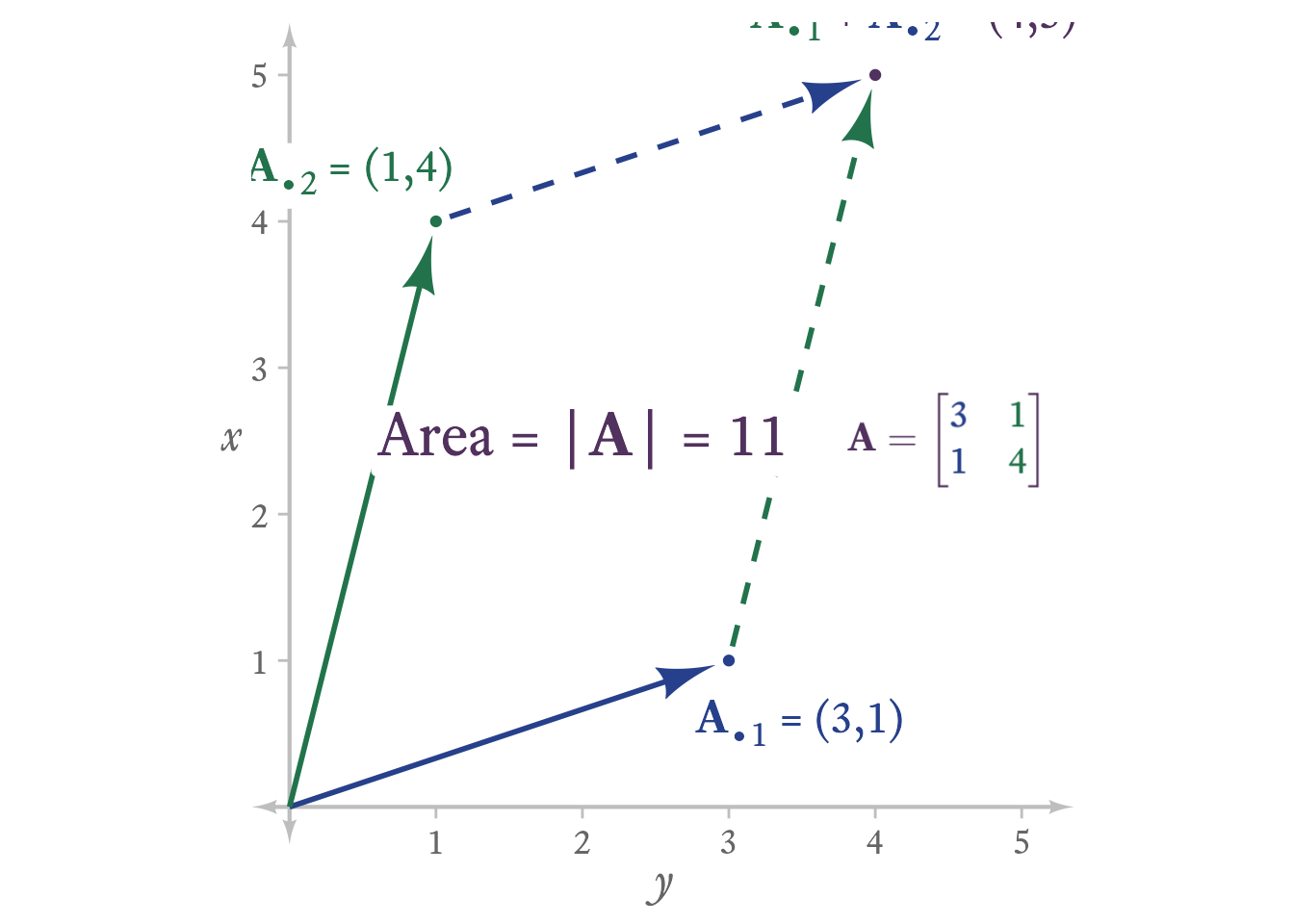
If a matrix is square, one can calculate its determinant. The determinant is a property of a square matrix indicates important information about the matrix. In a k × k matrix, it is equal to the volume of the k-dimensional parallelpiped spanned by its column (or row) vectors.
Consider the the matrix A:
\mathbf{A}=\begin{bmatrix} 3 & 1\\ 1 & 4 \end{bmatrix}
In Figure 6.2, the 2 column vectors of A and their sum form a parallelogram. The area of this parallelogram is equal to the determinant of A.
To calculate a determinant, it is useful to introduce some vocabulary. The minor of a matrix A at element (i, j) is the determinant of the submatrix of A after row i and column j have been deleted.
The determinant of matrix can be calculated like so:
- Take the first column vector of A. Each element can be called ai1.
- Multiply each element in ai1, by its minor and by −1i
- Add the resulting products.
Note that this method of calculating the determinant is recursive, meaning that the method calls on itself. In this case, calculating a determinant of a matrix requires calculating the determinant of a smaller submatrix. Thus, the determinant of a k by k matrix requires the calculation of a k − 1 by k − 1 matrix, which requires the calculation of a k − 2 by k − 2 matrix, and so on, and so on. For this method to find a stopping point, we have to assume that the determinant of a 1 by 1 matrix is the 1 by 1 matrix itself.
For the purpose of illustration only, here is a recursive function for calculating a determinant.
my_determinant <- function(A) {
  # If A is a 1 by 1 matrix, return A
  if (nrow(A) == 1 && ncol(A) == 1) {
    return(A[1, 1, drop = TRUE])
  }

  # Get first column of A
  A_o1 <- A[, 1]
  # Row Index
  i <- seq_along(A_o1)

  map2_dbl(A_o1, i, \(a, i) {
    # subtract even rows
    pm <- ifelse(i %% 2 == 0, -1, 1)
    a * pm * my_determinant(A[-i, -1, drop = FALSE])
  }) %>%
  sum()
}

my_determinant(A)
[1] 11Compared to det, the actual R function to calculate the determinant of a matrix, my recursive function is very slow. The det function hands that task over to a much faster algorithm that runs in the C programming language, which is generally faster than R. For a small matrix like A, the speed difference hardly matters. For repeated calculations with large matrices (e.g., in 3D graphics), it makes a huge difference.
det(A)[1] 116.11 Eigenvectors and Eigenvalues
Consider this equation showing the relationship between a square matrix \mathbf{A}, a column vector \vec{x}, and a column vector \vec{b}:
\mathbf{A}\vec{x}=\vec{b}
As explained in 3Blue1Brown’s wonderful Essence of Linear Algebra series, we can think of the square matrix \mathbf{A} as a mechanism for scaling and rotating vector \vec{x} to become vector \vec{b}.
Is there a non-zero vector \vec{v} that \mathbf{A} will scale but not rotate? If so, \vec{v} is an eigenvector. The value \lambda by which \vec{v} is scaled is the eigenvalue.
\mathbf{A}\vec{v}=\lambda\vec{v}
Every eigenvector that exists for matrix \mathbf{A}, is accompanied by an infinite number of parallel vectors of varying lengths that are also eigenvectors. Thus, we focus on the unit eigenvectors and their accompanying eigenvalues.
Eigenvectors and eigenvalues are extremely important concepts in a wide variety of applications in many disciplines, including psychometrics. Via principal components analysis, eigenvectors can help us summarize a large number of variables with a much smaller set of variables.
6.11.1 Eigenvectors and Eigenvalues in R
Suppose that matrix \mathbf{A} is a correlation matrix:
\mathbf{A}=\begin{bmatrix} 1 & 0.8 & 0.5\\ 0.8 & 1 & 0.4\\ 0.5 & 0.4 & 1 \end{bmatrix}
Because \mathbf{A} is a 3 × 3 matrix, there are three orthogonal unit vectors that are eigenvectors, \vec{v}_1, \vec{v}_2, and \vec{v}_3. We will collect the three eigenvectors as columns of matrix \mathbf{V}:
\mathbf{V}= \begin{bmatrix} \overset{\vec{v}_1}{.63} & \overset{\vec{v}_2}{.25} & \overset{\vec{v}_3}{.74}\\ .61 & .44 & −.67\\ .48 & −.87 & −.13 \end{bmatrix}
The three eigenvalues of \mathbf{A} are collected in the vector \vec{\lambda}:
\vec{\lambda} = (2.15,0.66,0.19)
\begin{aligned} \mathbf{AV}&=\mathtt{diag}\left(\vec{\lambda}\right)\mathbf{V}\\ \mathbf{AV}-\mathtt{diag}\left(\vec{\lambda}\right)\mathbf{V}&=\mathbf{0}\\ \left(\mathbf{A}-\mathtt{diag}\left(\vec{\lambda}\right)\right)\mathbf{V}&=\mathbf{0} \end{aligned}
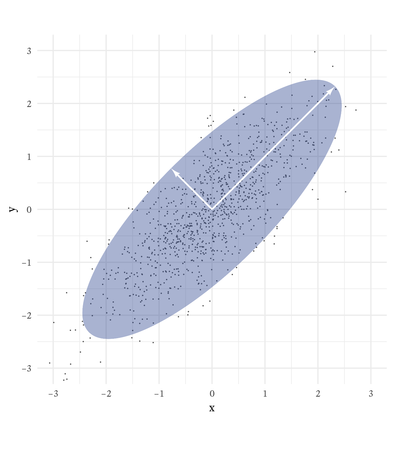
Suppose we generate multivariate normal data with population correlations equal to matrix \mathbf{A}. Plotted in three dimensions, the data would have the shape of an ellipsoid. As seen in Figure 6.3, the eigenvectors of \mathbf{A}, scaled by the square roots of the eigenvalues align with and are proportional to the principal axes of the ellipsoid that contains 95% of the data.
For symmetric matrices (e.g., correlation and covariance matrices), eigenvectors are orthogonal.
Eigenvalues and eigenvectors are essential ingredients in principal component analysis, a useful data-reduction technique. Principal component analysis allow us to summarize many variables in a way that minimizes information loss. To take a simple example, if we measure the size of people’s right and left feet, we would have two scores per person. The two scores are highly correlated because the left foot and right foot are nearly the same size in most people. However, for some people the size difference is notable.
Principal components analysis transforms the two correlated variables into two uncorrelated variables, one for the overall size of the foot and one for the difference between the two feet. Thus, we still have 2 scores, but the first score, the overall foot score, is the primary score that most people want to know. The second score, the difference between foot sizes, is important for some people, but is trivially small for most people. In general, principal components reorganizes the data so that the information from many scores can be succinctly summarized with a small number of scores.
The eigenvalues sum to the 2 (then number of variables being summarized) and are proportional to the variance explained by their respective principal components.
Eigenvectors have a magnitude of 1, but if they are scaled by the square root of the eigenvalues (and by the appropriate z-score), they become the principal axes of the ellipse that contains the 95% of the data (See Figure 6.4). Why the square root of the eigenvalues? Because eigenvalues are variances of the (unstandardized) principal components. The square root of eigenvalues are principal components’ standard deviations.