10  Distributions

Continuous

10.1 Probability Density Functions

Although there are many more discrete distribution families, we will now consider some continuous distribution families. Most of what we have learned about discrete distributions applies to continuous distributions. However, there is a need of a name change for the probability mass function. In a discrete distribution, we can calculate an actual probability for a particular value in the sample space. In continuous distributions, doing so can be tricky. We can always calculate the probability that a score in a particular interval will occur. However, in continuous distributions, the intervals can become very small, approaching a width of 0. When that happens, the probability associated with that interval also approaches 0. Yet, some parts of the distribution are more probable than others. Therefore, we need a measure of probability that tells us the probability of a value relative to other values: the probability density function

The probability density function is function that can show relative likelihoods of sample space elements of a continuous random variable.

Considering the entire sample space of a discrete distribution, all of the associated probabilities from the probability mass function sum to 1. In a probability density function, it is the area under the curve that must sum to 1. That is, there is a 100% probability that a value generated by the random variable will be somewhere under the curve. There is nowhere else for it to go!

However, unlike probability mass functions, probability density functions do not generate probabilities. Remember, the probability of any value in the sample space of a continuous variable is infinitesimal. We can only compare the probabilities to each other. To see this, compare the discrete uniform distribution and continuous uniform distribution in Figure 9.2. Both distributions range from 1 to 4. In the discrete distribution, there are 4 points, each with a probability of ¼. It is easy to see that these 4 probabilities of ¼ sum to 1. Because of the scale of the figure, it is not easy to see exactly how high the probability density function is in the continuous distribution. It happens to be ⅓. Why? First, it does not mean that each value has a ⅓ probability. There are an infinite number of points between 1 and 4 and it would be absurd if each of them had a ⅓ probability. The distance between 1 and 4 is 3. In order for the rectangle to have an area of 1, its height must be ⅓. What does that ⅓ mean, then? In the case of a single value in the sample space, it does not mean much at all. It is simply a value that we can compare to other values in the sample space. It could be scaled to any value, but for the sake of convenience it is scaled such that the area under the curve is 1.

Note that some probability density functions can produce values greater than 1. If the range of a continuous uniform distribution is less than 1, at least some portions of the curve must be greater than 1 to make the area under the curve equal 1. For example, if the bounds of a continuous distribution are 0 and ⅓, the average height of the probability density function would need to be 3 so that the total area is equal to 1.

10.2 Continuous Uniform Distributions

Feature	Symbol
Lower Bound	$a \in (-\infty,\infty)$
Upper Bound	$b \in (a,\infty)$
Sample Space	$x \in \lbrack a,b\rbrack$
Mean	$\mu = \frac{a+b}{2}$
Variance	$\sigma^2 = \frac{(b-a)^2-1}{12}$
Skewness	$\gamma_1 = 0$
Kurtosis	$\gamma_2 = -\frac{6}{5}$
Probability Density Function	$f_X(x;a,b) = \frac{1}{b-a}$
Cumulative Distribution Function	$F_X(x;a,b) = \frac{x-a}{b-a}$

Table 10.1: Features of Continuous Discrete Distributions

Unlike the discrete uniform distribution, the uniform distribution is continuous.¹ In both distributions, there is an upper and lower bound and all members of the sample space are equally probable.

¹ For the sake of clarity, the uniform distribution is often referred to as the continuous uniform distribution.

10.2.1 Generating random samples from the continuous uniform distribution

To generate a sample of $n$ numbers with a continuous uniform distribution between $a$ and $b$, use the runif function like so:

# Sample size
n <- 1000
# Lower and upper bounds
a <- 10
b <- 30
# Sample
x <- runif(n, min = a, max = b)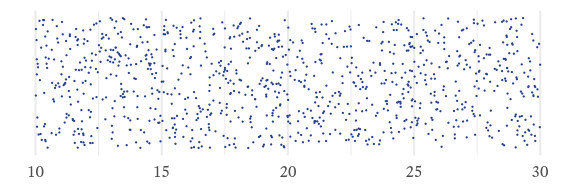

Figure 10.1: Random sample (n = 1000) of a continuous uniform distribution between 10 and 30. Points are randomly jittered to show the distribution more clearly.

R Code for Figure 10.1

# Plot
tibble(x) %>% 
ggplot(aes(x, y = 0.5)) + 
  geom_jitter(size = 0.5, 
              pch = 16,
              color = myfills[1], 
              height = 0.45) +
  scale_x_continuous(NULL) +
  scale_y_continuous(NULL, 
                     breaks = NULL, 
                     limits = c(0,1), expand = expansion()) + 
  theme_minimal(base_family = bfont, base_size = bsize)

10.2.1.1 Using the continuous uniform distribution to generate random samples from other distributions

Uniform distributions can begin and end at any real number but one member of the uniform distribution family is particularly important—the uniform distribution between 0 and 1. If you need to use Excel instead of a statistical package, you can use this distribution to generate random numbers from many other distributions.

The cumulative distribution function of any continuous distribution converts into a continuous uniform distribution. A distribution’s quantile function converts a continuous uniform distribution into that distribution. Most of the time, this process also works for discrete distributions. This process is particularly useful for generating random numbers with an unusual distribution. If the distribution’s quantile function is known, a sample with a continuous uniform distribution can easily be generated and converted.

For example, the RAND function in Excel generates random numbers between 0 and 1 with a continuous uniform distribution. The BINOM.INV function is the binomial distribution’s quantile function. Suppose that $n$ (number of Bernoulli trials) is 5 and $p$ (probability of success on each Bernoulli trial) is 0.6. A randomly generated number from the binomial distribution with $n=5$ and $p=0.6$ is generated like so:

=BINOM.INV(5,0.6,RAND())

Excel has quantile functions for many distributions (e.g., BETA.INV, BINOM.INV, CHISQ.INV, F.INV, GAMMA.INV, LOGNORM.INV, NORM.INV, T.INV). This method of combining RAND and a quantile function works reasonably well in Excel for quick-and-dirty projects, but when high levels of accuracy are needed, random samples should be generated in a dedicated statistical program like R, Python (via the numpy package), Julia, STATA, SAS, or SPSS.

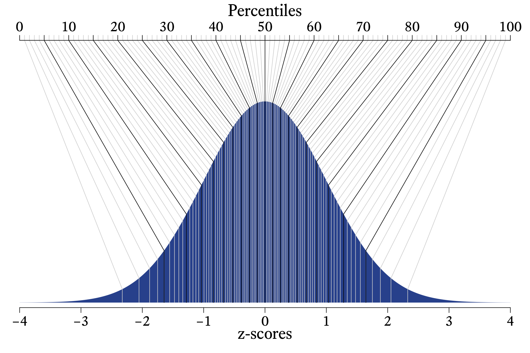
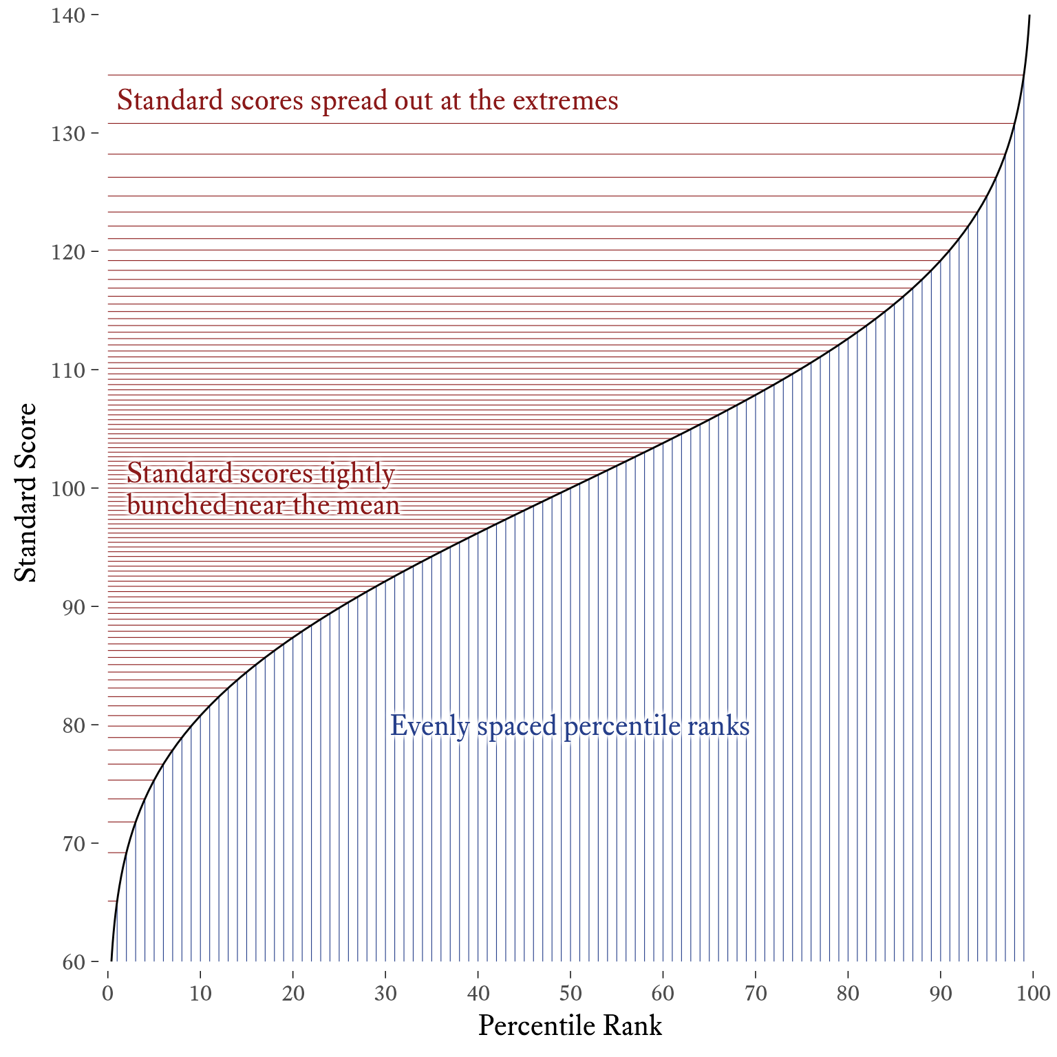
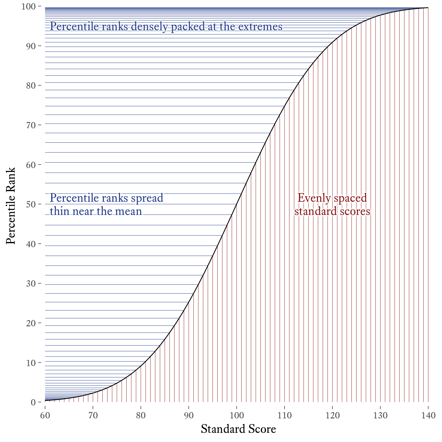
10.3 Normal Distributions

(Unfinished)

Feature	Symbol
Sample Space	$x \in (-\infty,\infty)$
Mean	$\mu = \mathcal{E}\left(X\right)$
Variance	$\sigma^2 = \mathcal{E}\left(\left(X - \mu\right)^2\right)$
Skewness	$\gamma_1 = 0$
Kurtosis	$\gamma_2 = 0$
Probability Density Function	$f_X(x;\mu,\sigma^2) = \frac{1}{\sqrt{2 \pi \sigma ^ 2}} e^{-\frac{1}{2}\left(\frac{x-\mu}{\sigma}\right)^2}$
Cumulative Distribution Function	$F_X(x;\mu,\sigma^2) = \frac{1}{\sqrt{2\pi\sigma^2}} {\displaystyle \int_{-\infty}^{x} e ^ {-\frac{1}{2}\left(\frac{x-\mu}{\sigma}\right)^2}dx}$

Table 10.2: Features of Normal Distributions

Figure 10.2: Carl Friedrich Gauss (1777–1855)
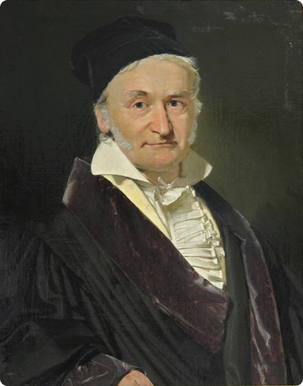
Image Credits

The normal distribution is sometimes called the Gaussian distribution after its discoverer, Carl Friedrich Gauss Figure 10.2. It is a small injustice that most people do not use Gauss’s name to refer to the normal distribution. Thankfully, Gauss is not exactly languishing in obscurity. He made so many discoveries that his name is all over mathematics and statistics.

The normal distribution is probably the most important distribution in statistics and in psychological assessment. In the absence of other information, assuming that an individual difference variable is normally distributed is a good bet. Not a sure bet, of course, but a good bet. Why? What is so special about the normal distribution?

To get a sense of the answer to this question, consider what happens to the binomial distribution as the number of events ($n$) increases. To make the example more concrete, let’s assume that we are tossing coins and counting the number of heads $(p=0.5)$. In Figure 10.3, the first plot shows the probability mass function for the number of heads when there is a single coin $(n=1)$). In the second plot, $n=2$ coins. That is, if we flip 2 coins, there will be 0, 1, or 2 heads. In each subsequent plot, we double the number of coins that we flip simultaneously. Even with as few as 4 coins, the distribution begins to resemble the normal distribution, although the resemblance is very rough. With 128 coins, however, the resemblance is very close.

Figure 10.3: The binomial distribution begins to resemble the normal distribution when the number of events is large.

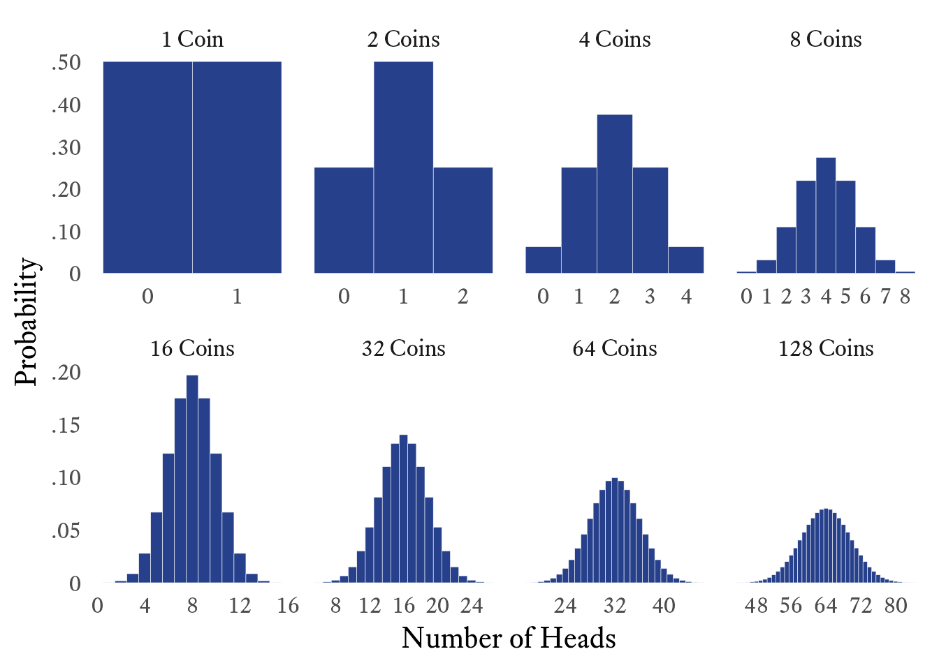
This resemblance to the normal distribution in the example is not coincidental to the fact that $p=0.5$, making the binomial distribution symmetric. If $p$ is extreme (close to 0 or 1), the binomial distribution is asymmetric. However, if $n$ is large enough, the binomial distribution eventually becomes very close to normal.

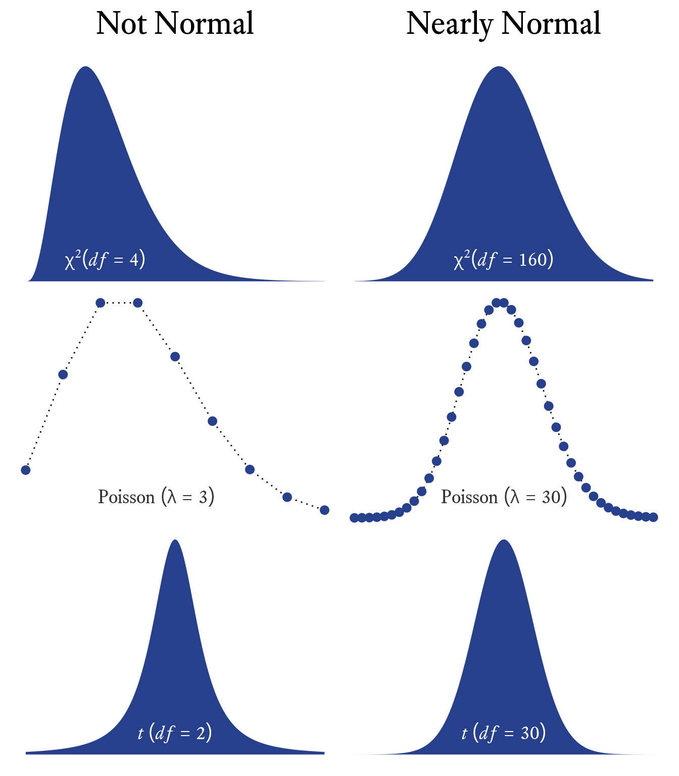
Many other distributions, such as the Poisson, Student’s T, F, and $\chi^2$ distributions, have distinctive shapes under some conditions but approximate the normal distribution in others (See Figure 10.4). Why? In the conditions in which non-normal distributions approximate the normal distribution, it is because, like in Figure 10.3, many independent events are summed.

Figure 10.4: Many distributions become nearly normal when their parameters are high.

10.3.1 Notation for Normal Variates

Statisticians write about variables with normal distributions so often that a compact notation for specifying a normal variable’s parameters was useful to develop. If I want to specify that $X$ is a normally variable with a mean of $\mu$ and a variance of $\sigma^2$, I will use this notation:

$$X \sim \mathcal{N}(\mu, \sigma^2)$$

Symbol	Meaning
$X$	A random variable.
$\sim$	Is distributed as
$\mathcal{N}$	Has a normal distribution
$\mu$	The population mean
$\sigma^2$	The population variance

Table 10.3: Features of Half-Normal Distributions

Many authors list the standard deviation $\sigma$ instead of the variance $\sigma^2$. When I specify normal distributions with specific means and variances, I will avoid ambiguity by always showing the variance as the standard deviation squared. For example, a normal variate with a mean of 10 and a standard deviation of 3 will be written as $X \sim \mathcal{N}(10,3^2)$.

Figure 10.5: Percentiles convert a distribution into a uniform distribution

Figure 10.6: Evenly spaced percentile ranks are associated with unevenly spaced scores.

Figure 10.7: Evenly spaced scores are associated with unevenly spaced percentiles

10.3.2 Half-Normal Distribution

(Unfinished)

Feature	Symbol
Sample Space	$x \in [\mu,\infty)$
Mu	$\mu \in (-\infty,\infty)$
Sigma	$\sigma \in [0,\infty)$
Mean	$\mu + \sigma\sqrt{\frac{2}{\pi}}$
Variance	$\sigma^2\left(1-\frac{2}{\pi}\right)$
Skewness	$\sqrt{2}(4-\pi)(\pi-2)^{-\frac{3}{2}}$
Kurtosis	$8(\pi-3)(\pi-2)^{-2}$
Probability Density Function	$f_X(x;\mu,\sigma) = \sqrt{\frac{2}{\pi \sigma ^ 2}} e^{-\frac{1}{2}\left(\frac{x-\mu}{\sigma}\right)^2}$
Cumulative Distribution Function	$F_X(x;\mu,\sigma) = \sqrt{\frac{2}{\pi\sigma}} {\displaystyle \int_{\mu}^{x} e ^ {-\frac{1}{2}\left(\frac{x-\mu}{\sigma}\right)^2}dx}$

Table 10.4: Features of Half-Normal Distributions

Figure 10.8: The half-normal distribution is the normal distribution with the left half of the distribution stacked on top of the right half of the distribution.

R Code for Figure 10.8

# Half normal distribution
xlim <- 4
n <- length(seq(-xlim, 0, 0.01))
t1 <- tibble(
  x = c(0,-xlim,
        seq(-xlim, 0, 0.01),
        0,
        0,
        seq(0, xlim, 0.01),
        xlim,
        0),
  y = c(0,
        0,
        dnorm(seq(-xlim, 0, 0.01)),
        0,
        0,
        dnorm(seq(0, xlim, 0.01)),
        0,
        0),
  side = c(rep(F, n + 3), rep(T, n + 3)),
  Type = 1
)
t2 <- t1 %>%
  mutate(y = if_else(side, y, 2 * y)) %>%
  mutate(x = abs(x),
         Type = 2)

bind_rows(t1, t2) %>%
  mutate(Type = factor(Type)) %>%
  ggplot(aes(x, y, fill = side)) +
  geom_polygon() +
  geom_text(
    data = tibble(
      x = 0,
      y = dnorm(0) * c(1, 2) + 0.14,
      Type = factor(c(1,2)),
      label = c(
        "Normal",
        "Half-Normal"),
      side = T),
    aes(label = label),
    family = bfont, fontface = "bold",
    size = ggtext_size(30), 
    vjust = 1
  ) +
  geom_richtext(
    data = tibble(
      x = 0,
      y = dnorm(0) * c(1, 2) + 0,
      Type = factor(c(1,2)),
      label = c(
        paste0("*X* ~ ",
               span_style("N", style = "font-family:'Lucida Calligraphy'"),
               "(*",
               span_style("&mu;", "font-family:serif;"),
               "*, *",
               span_style("&sigma;","font-family:serif;"),
               "*<sup>2</sup>)"),
        paste0("*X* ~ |",
               span_style("N", style = "font-family:'Lucida Calligraphy'"),
               "(0, *",
               span_style("&sigma;","font-family:serif;"),
               "*<sup>2</sup>)| + *",
               span_style("&mu;","font-family:serif;"),
               "*")),
      side = T),
    aes(label = label),
    family = c("Equity Text A"),
    size = ggtext_size(30), 
    vjust = 0, 
    label.padding = unit(0,"lines"), 
    label.color = NA,
    fill = NA) +
  theme_void(base_size = 30,
                base_family = bfont) +
  theme(
    legend.position = "none",
    strip.text = element_blank()
  ) +
  scale_fill_manual(values = myfills) +
  facet_grid(rows = vars(Type), space = "free_y", scales = "free_y") 

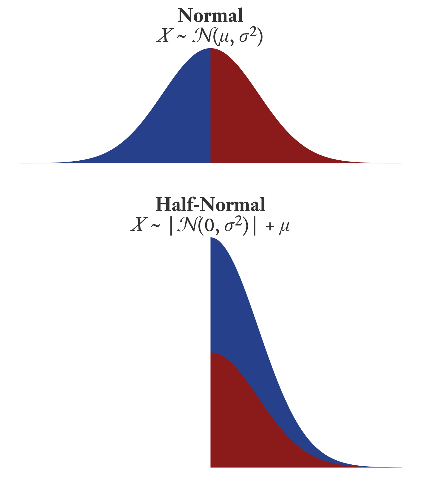
Suppose that $X$ is a normally distributed variable such that

$$X \sim \mathcal{N}(\mu, \sigma^2)$$

Variable $Y$ then has a half-normal distribution such that $Y = |X-\mu|+\mu$. In other words, imagine that a normal distribution is folded at the mean with the left half of the distribution now stacked on top of the right half of the distribution (See Figure 10.8).

10.3.3 Truncated Normal Distributions

(Unfinished)

10.3.4 Multivariate Normal Distributions

(Unfinished)

10.4 Chi Square Distributions

(Unfinished)

Feature	Symbol
Sample Space	$x \in [0,\infty)$
Degrees of freedom	$\nu \in [0,\infty)$
Mean	$\nu$
Variance	$2\nu$
Skewness	$\sqrt{8/\nu}$
Kurtosis	$12/\nu$
Probability Density Function	$f_X(x;\nu) = \frac{x^{\nu/2-1}}{2^{\nu/2}\;\Gamma(\nu/2)\,\sqrt{e^x}}$
Cumulative Distribution Function	$F_X(x;\nu) = \frac{\gamma\left(\frac{\nu}{2},\frac{x}{2}\right)}{\Gamma(\nu/2 )}$

Table 10.5: Features of Chi-Square Distributions

I have always thought that the $\chi^2$ distribution has an unusual name. The chi part is fine, but why square? Why not call it the $\chi$ distribution?² As it turns out, the $\chi^2$ distribution is formed from squared quantities.

² Actually, there is a $\chi$ distribution. It is simply the square root of the $\chi^2$ distribution. The half-normal distribution happens to be a $\chi$ distribution with 1 degree of freedom.

Notation note: A $\chi^2$ distribution with $\nu$ degrees of freedom can be written as $\chi^2_\nu$ or $\chi^2(\nu)$.

The $\chi^2$ distribution has a straightforward relationship with the normal distribution. It is the sum of multiple independent squared normal variates. That is, suppose $z$ is a standard normal variate:

$$z\sim\mathcal{N}(0,1^2)$$

In this case, $z^2$ has a $\chi^2$ distribution with 1 degree of freedom $(\nu)$:

$$z^2\sim \chi^2_1$$

If $z_1$ and $z_2$ are independent standard normal variates, the sum of their squares has a $\chi^2$ distribution with 2 degrees of freedom:

$$z_1^2+z_2^2 \sim \chi^2_2$$

If $\{z_1,z_2,\ldots,z_{\nu} \}$ is a series of $\nu$ independent standard normal variates, the sum of their squares has a $\chi^2$ distribution with $\nu$ degrees of freedom:

$$\sum^\nu_{i=1}{z_i^2} \sim \chi^2_\nu$$

10.4.1 Clinical Uses of the $\chi^2$ distribution

The $\chi^2$ distribution has many applications, but the mostly likely of these to be used in psychological assessment is the $\chi^2$ Test of Goodness of Fit and the $\chi^2$ Test of Independence.

The $\chi^2$ Test of Goodness of Fit tells us if observed frequencies of events differ from expected frequencies. Suppose we suspect that a child’s temper tantrums are more likely to occur on weekdays than on weekends. The child’s mother has kept a record of each tantrum for the past year and was able to count the frequency of tantrums. If tantrums were equally likely to occur on any day, 5 of 7 tantrums should occur on weekdays, and 2 of 7 tantrums should occur on weekends. The observed frequencies are compared with the expected frequencies below.

$$\begin{array}{r|c|c|c} & \text{Weekday} & \text{Weekend} & \text{Total} \\ \hline \text{Observed Frequency}\, (o) & 14 & 14 & n=28\\ \text{Expected Proportion}\,(p) & \frac{5}{7} & \frac{2}{7} & 1\\ \text{Expected Frequency}\, (e = np)& 28\times \frac{5}{7}= 20& 28\times \frac{2}{7}= 8& 28\\ \text{Difference}\,(o-e) & -6 & 6\\ \frac{(o-e)^2}{e} & 1.8 & 4.5 & \chi^2 = 6.3 \end{array}$$

In the table above, if the observed frequencies $(o_i)$ are compared to their respective expected frequencies $(e_i)$, then:

$$\chi^2_{k-1}=\sum_{i=1}^k{\frac{(o_i-e_i)^2}{e_i}}=6.3$$

Using the $\chi^2$ cumulative distribution function, we find that the probability of observing the frequencies listed is low under the assumption that tantrums are equally likely each day.

observed_frequencies <- c(Weekday = 14, Weekend = 14)
expected_probabilities <- c(Weekday = 5, Weekend = 2) / 7

fit <- chisq.test(x = observed_frequencies, 
                  p = expected_probabilities)
fit

    Chi-squared test for given probabilities

data:  observed_frequencies
X-squared = 6.3, df = 1, p-value = 0.01207

# View expected frequencies and residuals
broom::augment(fit)

# A tibble: 2 × 6
  Var1    .observed .prop .expected .resid .std.resid
  <fct>       <dbl> <dbl>     <dbl>  <dbl>      <dbl>
1 Weekday        14   0.5        20  -1.34      -2.51
2 Weekend        14   0.5         8   2.12       2.51

d_table <- tibble(A = rbinom(100, 1, 0.5)) |> 
  mutate(B = rbinom(100, 1, (A + 0.5) / 3)) |>
  table() 

d_table |> 
  as_tibble() |> 
  pivot_wider(names_from = A,
              values_from = n) |> 
knitr::kable(align = "lcc") |>
  kableExtra::kable_styling(bootstrap_options = "basic") |>
  kableExtra::collapse_rows() |> 
  kableExtra::add_header_above(header = c(` ` = 1, A = 2)) |> 
  html_table_width(400)

	A
B	0	1
0	47	21
1	11

fit <- chisq.test(d_table)

broom::augment(fit)

# A tibble: 4 × 9
  A     B     .observed .prop .row.prop .col.prop .expected .resid .std.resid
  <fct> <fct>     <int> <dbl>     <dbl>     <dbl>     <dbl>  <dbl>      <dbl>
1 0     0            47  0.47     0.810     0.691      39.4   1.20       3.28
2 1     0            21  0.21     0.5       0.309      28.6  -1.41      -3.28
3 0     1            11  0.11     0.190     0.344      18.6  -1.75      -3.28
4 1     1            21  0.21     0.5       0.656      13.4   2.06       3.28

10.5 Student’s t Distributions

Feature	Symbol
Sample Space	$x \in (-\infty,\infty)$
Degrees of Freedom	$\nu \in (0,\infty)$
Mean	$\left\{ \begin{array}{ll} 0 & \nu \gt 1 \\ \text{Undefined} & \nu \le 1 \\ \end{array} \right.$
Variance	$\left\{ \begin{array}{ll} \frac{\nu}{\nu-2} & \nu\gt 2 \\ \infty & 1 \lt \nu \le 2\\ \text{Undefined} & \nu \le 1 \\ \end{array} \right.$
Skewness	$\left\{ \begin{array}{ll} 0 & \nu \gt 3 \\ \text{Undefined} & \nu \le 3 \\ \end{array} \right.$
Kurtosis	$\left\{ \begin{array}{ll} \frac{6}{\nu-4} & \nu \gt 4 \\ \infty & 2 \lt \nu \le 4\\ \text{Undefined} & \nu \le 2 \\ \end{array} \right.$
Probability Density Function	$f_X(x; \nu) = \frac{\Gamma(\frac{\nu+1}{2})} {\sqrt{\nu\pi}\,\Gamma(\frac{\nu}{2})} \left(1+\frac{x^2}{\nu} \right)^{-\frac{\nu+1}{2}}$
Cumulative Distribution Function	$F_X(x; \nu)=\frac{1}{2} + x \Gamma \left( \frac{\nu+1}{2} \right) \frac{\phantom{\,}_{2}F_1 \left(\frac{1}{2},\frac{\nu+1}{2};\frac{3}{2};-\frac{x^2}{\nu} \right)} {\sqrt{\pi\nu}\,\Gamma \left(\frac{\nu}{2}\right)}$

Table 10.6: Features of Student’s t Distributions
Notation note: $\Gamma$ is the gamma function. $_2F_1$ is the hypergeometric function.

Figure 10.9: “Student” statistician, William Sealy Gosset (1876–1937)
Image Credit

(Unfinished)

Guinness Beer gets free advertisement every time the origin story of the Student t distribution is retold, and statisticians retell the story often. The fact that the original purpose of the t distribution was to brew better beer seems too good to be true.

William Sealy Gosset (1876–1937), self-trained statistician and head brewer at Guinness Brewery in Dublin, continually experimented on small batches to improve and standardize the brewing process. With some help from statistician Karl Pearson, Gosset used then-current statistical methods to analyze his experimental results. Gosset found that Pearson’s methods required small adjustments when applied to small samples. With Pearson’s help and encouragement (and later from Ronald Fisher), Gosset published a series of innovative papers about a wide range of statistical methods, including the t distribution, which can be used to describe the distribution of sample means.

Worried about having its trade secrets divulged, Guinness did not allow its employees to publish scientific papers related to their work at Guinness. Thus, Gosset published his papers under the pseudonym, “A Student.” The straightforward names of most statistical concepts need no historical treatment. Few of us who regularly use the Bernoulli, Pareto, Cauchy, and Gumbell distributions could tell you anything about the people who discovered them. But the oddly named “Student’s t distribution” cries out for explanation. Thus, in the long run, it was Gosset’s anonymity that made him famous.

Figure 10.10: The t distribution approaches the standard normal distribution as the degrees of freedom (df) parameter increases.

R Code for Figure 10.10

# The t distribution approaches the normal distribution
d <- crossing(x = seq(-6,6,0.02), 
         df = c(seq(1,15,1),
                seq(20,45,5),
                seq(50,100,10),
                seq(200,700,100))) %>%
  mutate(y = dt(x,df),
         Normal = dnorm(x)) 

t_size <- 40

d_label <- d %>% 
  select(df) %>% 
  unique() %>% 
  mutate(lb = qt(.025, df),
         ub = qt(0.975, df)) %>% 
  pivot_longer(c(lb, ub), values_to = "x", names_to = "bounds") %>% 
  mutate(label_x = signs::signs(x, accuracy = .01),
         y = 0,
         yend = dt(x, df))

p <- ggplot(d, aes(x, y)) + 
  geom_area(aes(y = Normal), alpha = 0.25, fill = myfills[1]) +
  geom_line() +
  geom_area(data = . %>% filter(x >= 1.96), 
            alpha = 0.25, 
            fill = myfills[1],
            aes(y = Normal)) +
  geom_area(data = . %>% filter(x <= -1.96), 
            alpha = 0.25, 
            fill = myfills[1],
            aes(y = Normal)) +
  geom_text(data = d_label, 
            aes(label = label_x), 
            family = bfont, 
            vjust = 1.25,
            size = ggtext_size(t_size)) + 
  geom_text(data = d_label %>% select(df) %>% unique,
            aes(x = 0, y = 0, label = paste0("df = ", df)), 
            vjust = 1.25, 
            family = bfont,
            size = ggtext_size(t_size)) + 
  geom_segment(data = d_label, aes(xend = x, yend = yend)) +
  transition_states(states = df, 
                    transition_length =  1, 
                    state_length = 2) +
  theme_void(base_size = t_size, base_family = bfont) +
  # labs(title = "df = {closest_state}") +
  annotate(x = qnorm(c(0.025, 0.975)), 
           y = 0, 
           label = signs::signs(qnorm(c(0.025, 0.975)), accuracy = .01), 
           geom = "text", 
           size = ggtext_size(t_size),
           color = myfills[1],
           vjust = 2.6, 
           family = bfont) + 
  coord_cartesian(xlim = c(-6,6), ylim = c(-.045, NA)) 

animate(p, 
        renderer = magick_renderer(), 
        device = "svglite", 
        fps = 2, 
        height = 6, 
        width = 10)
gganimate::anim_save("tdist_norm.gif")

10.5.1 The t distribution’s relationship Relationship to the normal distribution.

Suppose we have two independent standard normal variates $Z_0 \sim \mathcal{N}(0, 1^2)$ and $Z_1 \sim \mathcal{N}(0, 1^2)$.

A t distribution with one degree of freedom is created like so:

$$T_1 = z_0\sqrt{\frac{1}{z_1^2}}$$

A t distribution with two degrees of freedom is created like so:

$$T_2 = z_0\sqrt{\frac{2}{z_1^2 + z_2^2}}$$

Where $z_0$, $z_1$ and $z_2$ are independent standard normal variates.

A t distribution with $\nu$ degrees of freedom is created like so:

$$T_v = z_0\sqrt{\frac{\nu}{\sum_{i=1}^\nu z_i^2}}$$

The sum of $\nu$ squared standard normal variates $\left(\sum_{i=1}^\nu z_i^2\right)$ has a $\chi^2$ distribution with $\nu$ degrees of freedom, which has a mean of $\nu$. Therefore, $\sqrt{\frac{\nu}{\sum_{i=1}^\nu z_i^2}}$, on average, equals one. However, the expression $\sqrt{\frac{\nu}{\sum_{i=1}^\nu z_i^2}}$ has a variability approaches 0 as $\nu$ increases. When $\nu$ is high, $z_0$ is being multiplied by a value very close to 1. Thus, $T_\nu$ is nearly normal at high levels of $nu$.

10.6 Additional Distributions

10.6.1 F Distributions

Suppose that $X$ is the ratio of two independent $\chi^2$ variates $U_1$ and $U_2$ scaled by their degrees of freedom $\nu_1$ and $\nu_2$, respectively:

$$X=\frac{\frac{U_1}{\nu_1}}{\frac{U_2}{\nu_2}}$$

The random variate $X$ will have an $F$ distribution with parameters, $\nu_1$ and $\nu_2$.

The primary application of the $F$ distribution is to test the equality of variances in ANOVA. I am unaware of any direct applications of the F distribution in psychological assessment.

10.6.2 Weibull Distributions

How long do we have to wait before an event occurs? With Weibull distributions, we model wait times in which the probability of the event changes depending on how long we have waited. Some machines are designed to last a long time, but defects in a part might cause it fail quickly. If the machine is going to fail, it is likely to fail early. If the machine works flawlessly in the early period, we worry about it less. Of course, all physical objects wear out eventually, but a good design and regular maintenance might allow a machine to operate for decades. The longer machine has been working well, the less risk that it will irreparably fail on any particular day.

For some things, the risk of failure on any particular day becomes increasingly likely the longer it has been used. Biological aging causes increasing risk of death over time such that the historical records have no instances of anyone living beyond

For some events, there is a constant probability that the event will occur. For others, the probability is higher at first but becomes steadily less likely over time

the longer we wait the greater the probability will occur. For example, as animals age the probability of death accelerates such that beyond a certain age no individual as been observed to survive.

10.6.3 Unfinished

• Gumbel Distributions
• Beta Distributions
• Exponential Distributions
• Pareto Distributions